SQL COUNT, AVG, and SUM with GROUP BY: Syntax and Examples
For someone writing their first summary queries; every aggregate below is shown with the number it returns from the same five rows.
On this page
A report asks one question about a whole table at once: how many rows there are, what the average
is, what they add up to. COUNT() answers the first, AVG() the second and SUM() the third, each
collapsing many rows into one number. What separates them is how each one treats a missing value.
SELECT COUNT(*)       -- number of rows, NULL values included
FROM table_name;

SELECT AVG(column)    -- mean of the non-NULL values in the column
FROM table_name;

SELECT SUM(column)    -- total of the non-NULL values in the column
FROM table_name;
COUNT(*)counts input rows, so a row is counted even when every column in it isNULL[1].COUNT(column)counts only the rows in which that column is not null[1].AVG()computes the mean of the non-null input values[1], so the divisor is the count of those values rather than the number of rows[3].- Over an empty result,
SUM()andAVG()come back asNULLwhileCOUNT()comes back as 0[1].
What COUNT, AVG, and SUM do
| Function | What it returns | Common use case |
|---|---|---|
COUNT() | number of rows or values | how many orders, users, or events exist |
AVG() | average numeric value | average salary, score, or order size |
SUM() | total numeric value | total revenue, quantity, or hours |
All three are aggregate functions: they read a set of rows and return a single value for it. Written
with no GROUP BY, the set is the whole table, and the query gives back exactly one row. Written
with GROUP BY, the set is each group, and the query gives back one row per group. The same
functions serve both cases, so learning what they do on a whole table is most of the work. Each of
them also accepts DISTINCT, which removes repeated values before the function runs.
Every query below runs against the same five rows:
CREATE TABLE Employees (
    employee_id INT,
    first_name VARCHAR(50),
    last_name VARCHAR(50),
    salary INT,
    department VARCHAR(50)
);

INSERT INTO Employees (employee_id, first_name, last_name, salary, department)
VALUES
    (1, 'John', 'Doe', 50000, 'Sales'),
    (2, 'Jane', 'Doe', 60000, 'IT'),
    (3, 'Jim', 'Beam', 55000, 'Sales'),
    (4, 'Jack', 'Daniels', NULL, 'IT'),
    (5, 'Johnny', 'Walker', 65000, 'Finance');
Five employees in three departments, and one of them, Jack Daniels, has no salary on file. That single NULL is what every result below turns on, so it is worth keeping in view. A NULL value is a missing value rather than a zero, and each of the three functions acts on that difference in its own way.

SQL COUNT()
COUNT() counts rows or non-NULL values, depending on what you put in the parentheses.
COUNT(*) vs COUNT(column) vs COUNT(DISTINCT column)
SELECT COUNT(*) AS total_rows,
       COUNT(salary) AS rows_with_salary,
       COUNT(DISTINCT department) AS unique_departments
FROM Employees;
| total_rows | rows_with_salary | unique_departments |
|---|---|---|
| 5 | 4 | 3 |
Three forms, three answers, from one pass over five rows. COUNT(*) counts the rows themselves,
whatever they contain[1].
COUNT(salary) counts the rows in which that column has a value, so Jack Daniels is left out and
the answer is 4. COUNT(DISTINCT department) counts distinct non-null
values[2], so Sales appearing
twice does not make it two, and a department recorded as NULL would be counted in neither the
distinct list nor COUNT(department). Reach for that third form when the question is about distinct
values rather than rows, such as how many departments are represented rather than how many
employees.
COUNT(1) is not the faster form. The MySQL 8.4 manual states that InnoDB handles
SELECT COUNT(*) and SELECT COUNT(1) the same way and that there is no performance difference
between them[2]. Write
COUNT(*), which says "count the rows" to the next person reading the query.
SQL AVG() and SUM()
AVG() returns the arithmetic mean of a numeric column and SUM() its total, and both read only
the values that are there.
SELECT AVG(salary) AS average_salary,
       SUM(salary) AS total_salary
FROM Employees;
| average_salary | total_salary |
|---|---|
| 57500 | 230000 |
AVG() computes the mean of the non-null input
values[1], which leaves the missing
salary out of the divisor as well as the sum: 230000 divided by 4, not by 5. Had the row counted as
a zero, the answer would have been 46000. Those two numbers answer different questions, one about
the salaries on file and one about a salary of zero. To ask the second question, say so:
SELECT AVG(COALESCE(salary, 0)) AS average_salary_including_missing_values
FROM Employees;
| average_salary_including_missing_values |
|---|
| 46000 |
The divisor is 5 now, and the answer has changed by more than eleven thousand. COALESCE is also
the answer to the empty case, because SUM() and AVG() return NULL rather than 0 when no row
matches at all[1]:
SELECT SUM(salary) AS total_salary
FROM Employees
WHERE department = 'Legal';
| total_salary |
|---|
| NULL |
Wrap the call in COALESCE(SUM(salary), 0) when the report needs a zero on the empty case.
The type the average comes back in is where an integer column bites. SQL Server returns an int
from AVG() over an int column[3],
so the fractional part is dropped unless the column is cast first. PostgreSQL 17 returns numeric
from avg(integer) and keeps
it[1]. The salaries here divide
evenly, so both engines answer 57500.
AVG(DISTINCT salary) returns the same 57500 against these rows, because no two employees earn the
same amount and removing duplicates removes nothing. Reach for DISTINCT only when a repeated value
would distort the answer, as in the average of a price list where one price is quoted by twenty
suppliers.
Practice this: Lesson 6 of the SQL tutorial runs COUNT, SUM, AVG, MIN and MAX on a shop database in your browser, with checked exercises.
GROUP BY and HAVING with aggregate functions
Group by department
SELECT department,
       COUNT(*) AS employee_count,
       AVG(salary) AS average_salary,
       SUM(salary) AS total_salary
FROM Employees
GROUP BY department
ORDER BY total_salary DESC;
| department | employee_count | average_salary | total_salary |
|---|---|---|---|
| Sales | 2 | 52500 | 105000 |
| Finance | 1 | 65000 | 65000 |
| IT | 2 | 60000 | 60000 |
GROUP BY department split the five rows into three groups, and each function ran once per group.
IT is the group to read twice: COUNT(*) says two employees, while the average and the total are
built from the single IT salary that is not NULL. Keeping COUNT() beside the other two is a
habit worth having, because it tells the reader of the report how many rows each average and total
was built from. MIN() and MAX() belong in the same
SELECT list and skip NULL the same
way[2].
Filter groups with HAVING
SELECT department,
       COUNT(*) AS employee_count,
       AVG(salary) AS average_salary,
       SUM(salary) AS total_salary
FROM Employees
GROUP BY department
HAVING SUM(salary) > 60000
ORDER BY total_salary DESC;
| department | employee_count | average_salary | total_salary |
|---|---|---|---|
| Sales | 2 | 52500 | 105000 |
| Finance | 1 | 65000 | 65000 |
IT dropped out, because its total of 60000 is not greater than 60000. A filter that reads an
aggregate has to wait until the aggregate exists, which is what HAVING is for, and
SQL HAVING Clause walks through the rest of it.
A grouped query collapses its rows, and there is no way to keep a detail row beside the summary it
belongs to. That is the job of PARTITION BY: AVG(salary) OVER (PARTITION BY department) writes
each department's average next to every employee in it and returns all five rows. Use GROUP BY for
one row per group, and see Window Functions in SQL when the
detail rows have to survive.
Conditional aggregation with CASE
SELECT
    COUNT(*) AS employee_count,
    SUM(CASE WHEN department = 'Sales' THEN salary ELSE 0 END) AS sales_payroll,
    AVG(CASE WHEN department = 'IT' THEN salary END) AS it_average_salary
FROM Employees;
| employee_count | sales_payroll | it_average_salary |
|---|---|---|
| 5 | 105000 | 60000 |
Groups can also become columns instead of rows. The CASE inside SUM() turns every non-Sales
salary into a 0, which adds nothing to the payroll. The CASE inside AVG() has no ELSE, so
every non-IT row becomes NULL and drops out of the average entirely, leaving 60000 from the one IT
employee who has a salary. That difference between ELSE 0 and no ELSE decides whether the
excluded rows count in the divisor.
Common mistakes and performance tips
The habits that turn a correct-looking query into a wrong number, or into no answer at all:
- Reading
COUNT(*)as if it wereCOUNT(column), when the first counts rows and the second counts values. - Adding
DISTINCTbecause the number looked too big, without deciding whether the repeated values are duplicates or genuine data. - Forgetting that
SUM()andAVG()skipNULL, and then explaining an average nobody can reproduce by hand. - Reading a
SUM()of no rows as a total of zero, when it arrives asNULL. - Selecting a column that is neither grouped nor aggregated, which at least announces itself, since the query is rejected instead of answering.
The performance tip worth the space is where you put the filter. A condition that does not read an aggregate belongs in WHERE, where it removes rows before any grouping happens:
SELECT department, SUM(salary) AS total_salary
FROM Employees
WHERE salary > 0
GROUP BY department;
The three totals come back unchanged from the grouped query above. The only row this filter removes
is Jack Daniels, whose salary is NULL, because a comparison against NULL is unknown rather than
true and the row never reaches SUM(). The same condition written in HAVING would group all five
rows first and throw the work away afterwards. If you need a refresher on row filters and sort
order, see
SQL WHERE Clause, SQL ORDER BY,
and the broader SQL Aggregate Functions.
Use aggregate queries in DbSchema
DbSchema keeps the schema, the data and the SQL in one window, which shortens the loop between writing an aggregate and checking it against the rows it summarizes.
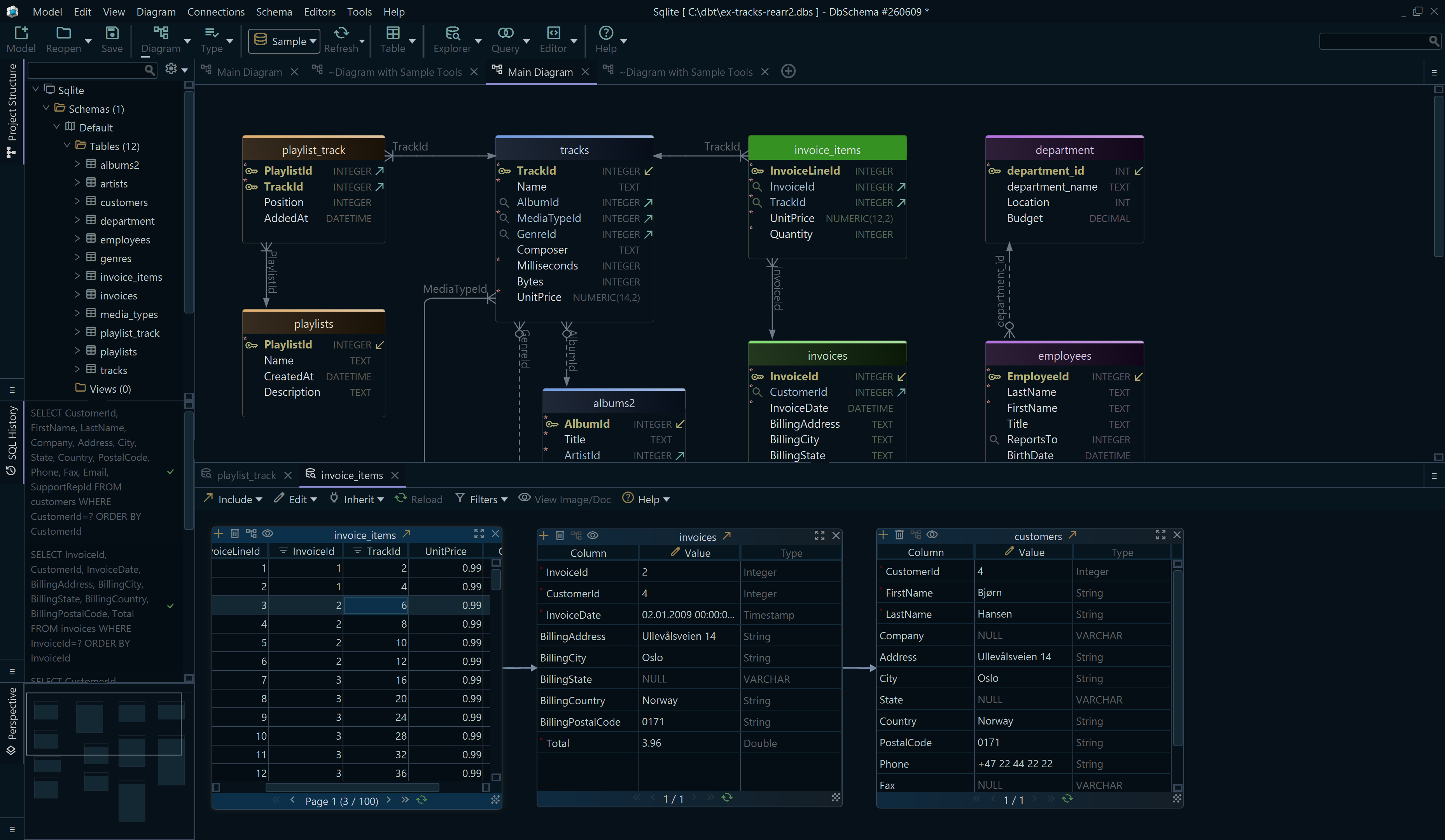
- Connect through the PostgreSQL JDBC driver or MySQL JDBC driver. DbSchema reverse-engineers the schema into a diagram, and the connection, the diagram and the SQL Editor are in the free Community Edition.
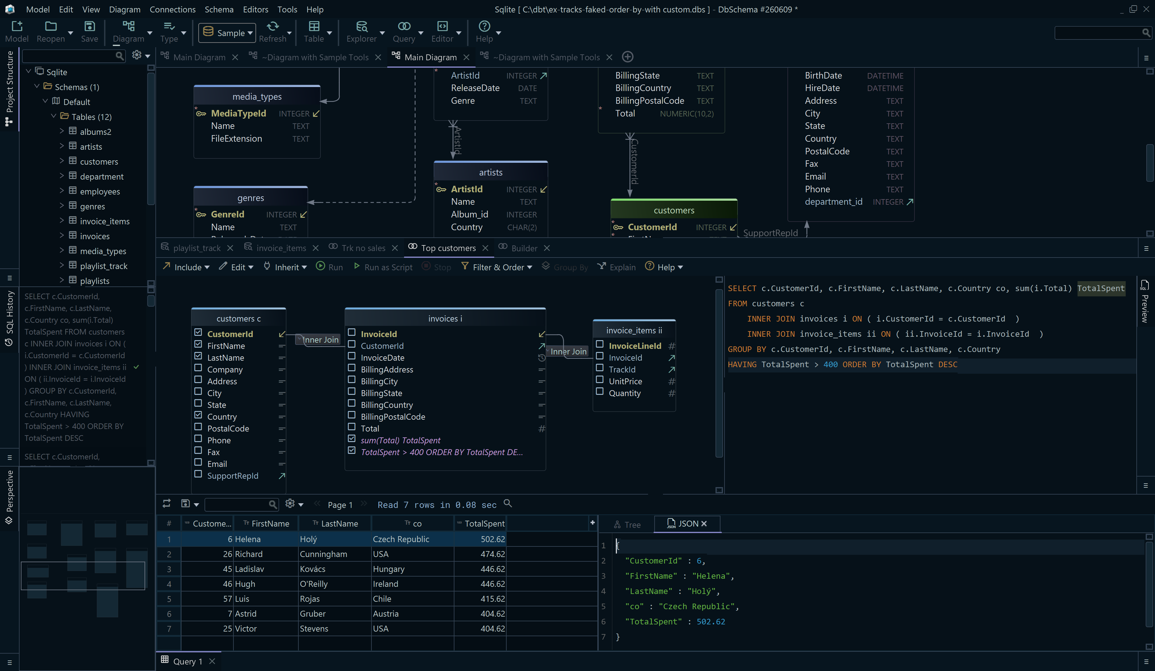
- Write the query in the SQL Editor and press Execute Query. The result comes back as a table, and the SQL History pane keeps every statement of the session, so you can step back to the version that gave the number you trusted.
- To build the grouped query without writing it, open the
Query Builder, turn on Group By mode from the toolbar, then
right-click a column and choose Aggregate to apply
MIN,MAX,SUM,AVGorCOUNT. DbSchema updates the generated SQL as you go. - To see the rows behind a group before you trust the total, open the Relational Data Editor and click from a parent row into its children. The Query Builder and the Relational Data Editor are in the Pro edition.
Both editors are saved inside the model file and reopen with it; the queries they generate run against the connected database.


Run COUNT(*) beside COUNT(column) on a table of your own that has a
nullable numeric column, and the two numbers say in a single row how much of the data is missing,
before any average from it is worth quoting. Download DbSchema at
https://dbschema.com/download.html to try that against your own
database: the connection, the diagram and the SQL Editor are in the free Community Edition, and the
Query Builder that writes the GROUP BY for you is in Pro.
Sources
Test your aggregate queries on real data
DbSchema connects to your database, reverse-engineers the schema, and runs COUNT, AVG and SUM in the SQL Editor. All three are in the free Community Edition.