Window Functions in SQL for Data Analysis
For SQL users comfortable with GROUP BY who now need a calculation per row instead of per group.
On this page
A running total that restarts with each group, the position of a row inside its group, the time between one row and the row before it: all three of those questions end the same way, because GROUP BY returns the number and takes away the rows. A window function computes across a set of rows related to the current row without grouping them into a single output row, so the rows keep their separate identities and the calculation arrives as one more column.
Filling the table with the DbSchema Data Generator
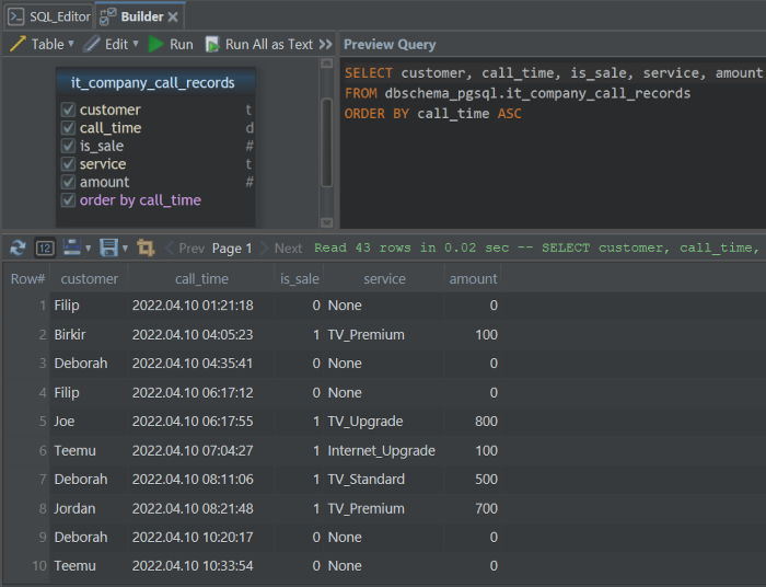
Every query below runs against one table of call records, where each row is one call to a customer that either ended in a sale or did not:
CREATE TABLE it_company_call_records (
  customer  text,
  call_time timestamp,
  is_sale   int,
  service   text,
  amount    int,
  PRIMARY KEY (customer, call_time, service)
);

INSERT INTO it_company_call_records VALUES
  ('Birkir', '2022-04-10 04:05:23', 1, 'TV_Premium',        100),
  ('Birkir', '2022-04-10 10:56:31', 1, 'Internet_Standard', 800),
  ('Jordan', '2022-04-10 08:21:48', 1, 'TV_Premium',        700),
  ('Jordan', '2022-04-10 12:42:45', 1, 'TV_Standard',       300),
  ('Jordan', '2022-04-11 09:01:55', 0, 'None',                0),
  ('Jordan', '2022-04-11 16:04:41', 1, 'Internet_Premium',  100),
  ('Jordan', '2022-04-12 07:10:50', 1, 'Internet_Premium',  800),
  ('Teemu',  '2022-04-10 07:04:27', 1, 'Internet_Upgrade',  100),
  ('Teemu',  '2022-04-10 10:33:54', 0, 'None',                0),
  ('Teemu',  '2022-04-10 14:36:27', 1, 'Internet_Standard', 500),
  ('Teemu',  '2022-04-11 02:53:46', 1, 'Internet_Upgrade',  600),
  ('Teemu',  '2022-04-13 22:46:25', 1, 'Internet_Standard', 700);
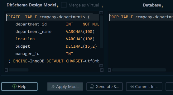
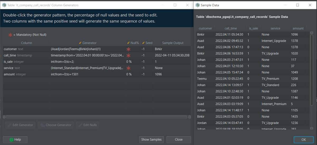
Twelve rows are enough to check a window function by eye, which is the point of using so few. For a table large enough to make the query plan interesting, the Data Generator in DbSchema fills it without a loading script: open it from Data Tools → Generate Random Data, or right-click the table header on the diagram and choose Generate Random Data. Set the number of rows per table, then double-click the table to open its column pattern editor, where each column gets a Pattern, a percentage of Nulls, and a Seed that makes the same sequence come back on the next run. The patterns are stored in the model file; clicking Generate is the step that writes rows into the database, and DbSchema asks first whether to drop what is already there. Generating random data for Postgres covers the pattern types in more detail. The Data Generator is a Pro feature.
What a window function keeps that GROUP BY throws away
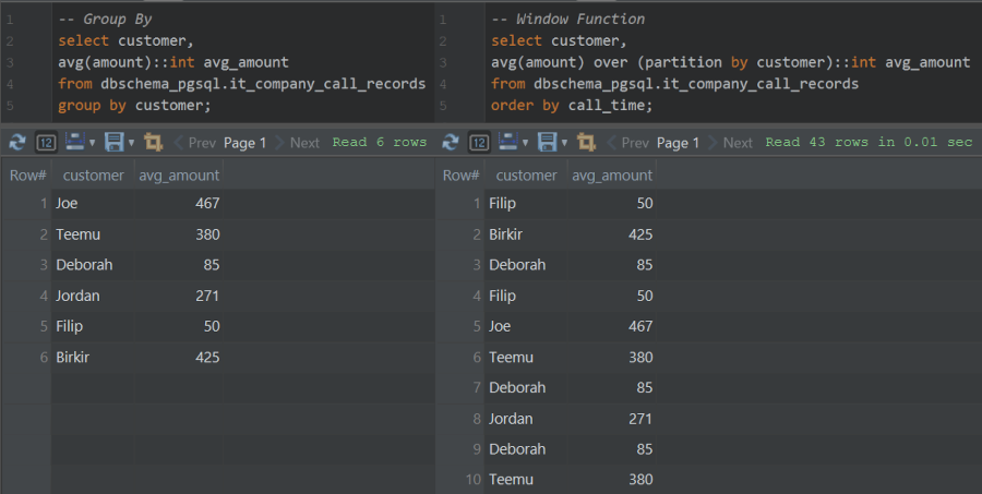
Ask for the average amount per customer with GROUP BY and you get three rows, one per customer, and the call records are gone. Every column that is not in the GROUP BY list or wrapped in an aggregate has nowhere to go, which is exactly what you want in a report and exactly what you do not want when the average is meant to sit next to each call as a comparison.
The same aggregate written as a window function returns twelve rows with the average repeated on each of them. PostgreSQL's own description of the difference is that window functions do not cause rows to become grouped into a single output row, so the rows retain their separate identities. Every column you already had stays available.
The window functions PostgreSQL provides
Three families cover almost everything you will write. Aggregate window functions are the aggregates you already use, evaluated over a set of rows instead of the whole group. Value window functions read a value out of another row in the same window: the row before, the row after, the first row. Rank window functions report the position of the current row among the rows it is being compared with.
| Aggregate | Value | Rank |
|---|---|---|
| SUM() | NTH_VALUE() | RANK() |
| COUNT() | LAG() | DENSE_RANK() |
| AVG() | LEAD() | ROW_NUMBER() |
| MIN() | FIRST_VALUE() | PERCENT_RANK() |
| MAX() | LAST_VALUE() | CUME_DIST() |
All of them are listed with their exact signatures in the PostgreSQL 18 window function reference. One restriction applies to every one of them: window functions are permitted only in the SELECT list and the ORDER BY clause, and are forbidden in GROUP BY, HAVING, and WHERE. Filtering on the result of a window function therefore means wrapping the query in a subquery and filtering outside it.
How OVER, PARTITION BY, and ORDER BY divide the rows
Say you want the time of each customer's first call, on every row belonging to that customer. FIRST_VALUE(call_time) on its own returns the first call in the whole table, twelve times over. OVER is where you say which rows count as the window, and it takes two parts.
PARTITION BY divides the rows into groups that share the same value of the expression, and the function is computed across the rows in the same partition as the current row. PARTITION BY customer therefore restarts the calculation for Birkir, Jordan, and Teemu separately. ORDER BY then decides which row comes first inside each partition, without which "first" means whichever row the plan happened to produce:
select customer, call_time,
       first_value(call_time) over (partition by customer order by call_time) as first_call_time
from it_company_call_records
order by customer, call_time;
| customer | call_time | first_call_time |
|---|---|---|
| Birkir | 2022-04-10 04:05:23 | 2022-04-10 04:05:23 |
| Birkir | 2022-04-10 10:56:31 | 2022-04-10 04:05:23 |
| Jordan | 2022-04-10 08:21:48 | 2022-04-10 08:21:48 |
| Jordan | 2022-04-10 12:42:45 | 2022-04-10 08:21:48 |
| Jordan | 2022-04-11 09:01:55 | 2022-04-10 08:21:48 |
| Jordan | 2022-04-11 16:04:41 | 2022-04-10 08:21:48 |
| Jordan | 2022-04-12 07:10:50 | 2022-04-10 08:21:48 |
| Teemu | 2022-04-10 07:04:27 | 2022-04-10 07:04:27 |
| Teemu | 2022-04-10 10:33:54 | 2022-04-10 07:04:27 |
| Teemu | 2022-04-10 14:36:27 | 2022-04-10 07:04:27 |
| Teemu | 2022-04-11 02:53:46 | 2022-04-10 07:04:27 |
| Teemu | 2022-04-13 22:46:25 | 2022-04-10 07:04:27 |
One detail separates FIRST_VALUE from its counterpart. FIRST_VALUE, LAST_VALUE, and NTH_VALUE read from the window frame rather than from the whole partition, and by default that frame ends at the current row and its peers. FIRST_VALUE is unaffected, since the frame always begins where the partition begins. LAST_VALUE is not: with the default frame it returns the current row, and reaching the partition's last row takes an explicit frame, ROWS BETWEEN UNBOUNDED PRECEDING AND UNBOUNDED FOLLOWING.
Feature engineering with window functions
A model wants one row per event with the context of the surrounding events attached to it: how much this customer had spent before this call, which call of the day this was, how long since the last one. Each of those is a column that describes the row in terms of its neighbors, and each of them is one window function away from the raw table.
Aggregating first and joining back is the alternative, and it costs a subquery plus a join per variable, all of which have to agree on the grouping. A join back on a key that turns out not to be unique also duplicates rows, quietly, in a dataset nobody counts twice. The window function version keeps the grain of the table, so the variables can be built one at a time in the same SELECT and read straight into a training set or a report.

Aggregate window functions over a partition
The running total of what a customer has spent, at each call, is SUM over a partition with an ORDER BY:
select customer, call_time, amount,
       sum(amount) over (partition by customer order by call_time) as cumulative_amount
from it_company_call_records
order by customer, call_time;
| customer | call_time | amount | cumulative_amount |
|---|---|---|---|
| Birkir | 2022-04-10 04:05:23 | 100 | 100 |
| Birkir | 2022-04-10 10:56:31 | 800 | 900 |
| Jordan | 2022-04-10 08:21:48 | 700 | 700 |
| Jordan | 2022-04-10 12:42:45 | 300 | 1000 |
| Jordan | 2022-04-11 09:01:55 | 0 | 1000 |
| Jordan | 2022-04-11 16:04:41 | 100 | 1100 |
| Jordan | 2022-04-12 07:10:50 | 800 | 1900 |
| Teemu | 2022-04-10 07:04:27 | 100 | 100 |
| Teemu | 2022-04-10 10:33:54 | 0 | 100 |
| Teemu | 2022-04-10 14:36:27 | 500 | 600 |
| Teemu | 2022-04-11 02:53:46 | 600 | 1200 |
| Teemu | 2022-04-13 22:46:25 | 700 | 1900 |
The ORDER BY is what turns the sum into a running one. With it, the default frame runs from the start of the partition up through the current row plus any following rows equal to the current row under that ORDER BY, which the PostgreSQL 18 tutorial spells out. Two calls at the same timestamp would therefore both show the total including both, and the fix is to order by something unique, here call_time plus service.
Adding a second expression to PARTITION BY resets the running total on each new day. The ::date cast reduces the timestamp to its date, so every call made on the same day by the same customer falls in one partition:
select customer, call_time, amount,
       sum(amount) over (partition by customer, call_time::date order by call_time)
         as cumulative_amount_daywise
from it_company_call_records
order by customer, call_time;
| customer | call_time | amount | cumulative_amount_daywise |
|---|---|---|---|
| Birkir | 2022-04-10 04:05:23 | 100 | 100 |
| Birkir | 2022-04-10 10:56:31 | 800 | 900 |
| Jordan | 2022-04-10 08:21:48 | 700 | 700 |
| Jordan | 2022-04-10 12:42:45 | 300 | 1000 |
| Jordan | 2022-04-11 09:01:55 | 0 | 0 |
| Jordan | 2022-04-11 16:04:41 | 100 | 100 |
| Jordan | 2022-04-12 07:10:50 | 800 | 800 |
| Teemu | 2022-04-10 07:04:27 | 100 | 100 |
| Teemu | 2022-04-10 10:33:54 | 0 | 100 |
| Teemu | 2022-04-10 14:36:27 | 500 | 600 |
| Teemu | 2022-04-11 02:53:46 | 600 | 600 |
| Teemu | 2022-04-13 22:46:25 | 700 | 700 |
When three columns share one window, name it once in a WINDOW clause and reference the name in each OVER. Dropping the ORDER BY inside the window changes the frame to the whole partition, which is what MAX, MIN, and COUNT want here: the day's largest sale, the day's first call, and the number of calls that day, repeated on every row of that day.
select customer, call_time, amount,
       max(amount)    over customer_date as max_amount_daywise,
       min(call_time) over customer_date as first_call_time_daywise,
       count(*)       over customer_date as total_calls_daywise
from it_company_call_records
window customer_date as (partition by customer, call_time::date)
order by customer, call_time;
| customer | call_time | amount | max_amount_daywise | first_call_time_daywise | total_calls_daywise |
|---|---|---|---|---|---|
| Birkir | 2022-04-10 04:05:23 | 100 | 800 | 2022-04-10 04:05:23 | 2 |
| Birkir | 2022-04-10 10:56:31 | 800 | 800 | 2022-04-10 04:05:23 | 2 |
| Jordan | 2022-04-10 08:21:48 | 700 | 700 | 2022-04-10 08:21:48 | 2 |
| Jordan | 2022-04-10 12:42:45 | 300 | 700 | 2022-04-10 08:21:48 | 2 |
| Jordan | 2022-04-11 09:01:55 | 0 | 100 | 2022-04-11 09:01:55 | 2 |
| Jordan | 2022-04-11 16:04:41 | 100 | 100 | 2022-04-11 09:01:55 | 2 |
| Jordan | 2022-04-12 07:10:50 | 800 | 800 | 2022-04-12 07:10:50 | 1 |
| Teemu | 2022-04-10 07:04:27 | 100 | 500 | 2022-04-10 07:04:27 | 3 |
| Teemu | 2022-04-10 10:33:54 | 0 | 500 | 2022-04-10 07:04:27 | 3 |
| Teemu | 2022-04-10 14:36:27 | 500 | 500 | 2022-04-10 07:04:27 | 3 |
| Teemu | 2022-04-11 02:53:46 | 600 | 600 | 2022-04-11 02:53:46 | 1 |
| Teemu | 2022-04-13 22:46:25 | 700 | 700 | 2022-04-13 22:46:25 | 1 |
MIN(call_time) answers the same question as FIRST_VALUE(call_time) did above and needs no ORDER BY to do it, because the smallest timestamp in the partition is the first call whichever order the rows arrive in.
ROW_NUMBER inside each partition
Once the partition is right, changing the question is mostly a matter of changing the function. ROW_NUMBER returns the number of the current row within its partition, counting from 1, so the call number per customer and the call number per customer per day are the same function over two different windows:
select customer, call_time,
       row_number() over (partition by customer order by call_time) as call_no_overall,
       row_number() over (partition by customer, call_time::date order by call_time)
         as call_no_daywise
from it_company_call_records
order by customer, call_time;
| customer | call_time | call_no_overall | call_no_daywise |
|---|---|---|---|
| Birkir | 2022-04-10 04:05:23 | 1 | 1 |
| Birkir | 2022-04-10 10:56:31 | 2 | 2 |
| Jordan | 2022-04-10 08:21:48 | 1 | 1 |
| Jordan | 2022-04-10 12:42:45 | 2 | 2 |
| Jordan | 2022-04-11 09:01:55 | 3 | 1 |
| Jordan | 2022-04-11 16:04:41 | 4 | 2 |
| Jordan | 2022-04-12 07:10:50 | 5 | 1 |
| Teemu | 2022-04-10 07:04:27 | 1 | 1 |
| Teemu | 2022-04-10 10:33:54 | 2 | 2 |
| Teemu | 2022-04-10 14:36:27 | 3 | 3 |
| Teemu | 2022-04-11 02:53:46 | 4 | 1 |
| Teemu | 2022-04-13 22:46:25 | 5 | 1 |
ROW_NUMBER never repeats a number inside a partition, even when two rows tie under the ORDER BY, and which of the tied rows gets the lower number is then unpredictable. Where the tie has to break the same way every time, add a column that makes the sort unique.
The same numbering is how you keep one row per group. A window function cannot appear in a WHERE clause, so the numbering goes in a subquery and the filter goes outside it:
select customer, call_time, amount
from (
  select customer, call_time, amount,
         row_number() over (partition by customer order by call_time desc) as rn
  from it_company_call_records
) ranked
where rn = 1
order by customer;
| customer | call_time | amount |
|---|---|---|
| Birkir | 2022-04-10 10:56:31 | 800 |
| Jordan | 2022-04-12 07:10:50 | 800 |
| Teemu | 2022-04-13 22:46:25 | 700 |
Sorting the window by call_time descending puts the latest call first in each partition, and rn = 1 keeps it, with every column of that row still attached.
Ranking customers with a CTE
Ranking customers by what they spent needs the total before it can rank anything, and a window function cannot be nested inside another one. A common table expression solves it in one statement: the WITH clause names a query, the main query reads it as a table, and the ranking runs over the totals:
with totals as (
  select customer, sum(amount) as customer_total_amount
  from it_company_call_records
  group by customer
)
select customer, customer_total_amount,
       dense_rank() over (order by customer_total_amount desc) as customer_rank,
       rank()       over (order by customer_total_amount desc) as customer_rank_with_gaps
from totals
order by customer_rank, customer;
| customer | customer_total_amount | customer_rank | customer_rank_with_gaps |
|---|---|---|---|
| Jordan | 1900 | 1 | 1 |
| Teemu | 1900 | 1 | 1 |
| Birkir | 900 | 2 | 3 |
Jordan and Teemu are tied, and the two functions disagree about what comes next. DENSE_RANK counts peer groups, so Birkir is second. RANK returns the row number of the first row in the peer group, which leaves a gap, so Birkir is third. Prefer DENSE_RANK when the rank is a label a person reads, and RANK when a gap after a tie is the answer you want, as it is in a leaderboard. There is no PARTITION BY here at all: leaving it out makes the whole result one window, which is what ranking every customer against every other customer means.
LAG and LEAD, one row back and one row forward
The last family reaches into another row of the same partition. LAG returns the value at the row a given number of rows before the current one, LEAD at the row after, and both return NULL when there is no such row. Three derived columns in one query: the service sold on the customer's first successful call, the minutes since their previous call, and whether a call that failed was followed by one that converted.
select customer, call_time, is_sale, service,
       first_value(service) over
         (partition by customer order by is_sale desc, call_time) as first_service,
       round(extract(epoch from (call_time -
         lag(call_time) over (partition by customer order by call_time))) / 60)
         as mins_since_last_call,
       case when is_sale = 0
             and lead(is_sale) over (partition by customer order by call_time) = 1
            then 'Yes' else 'No' end as nosale_to_sale
from it_company_call_records
order by customer, call_time;
| customer | call_time | is_sale | service | first_service | mins_since_last_call | nosale_to_sale |
|---|---|---|---|---|---|---|
| Birkir | 2022-04-10 04:05:23 | 1 | TV_Premium | TV_Premium | No | |
| Birkir | 2022-04-10 10:56:31 | 1 | Internet_Standard | TV_Premium | 411 | No |
| Jordan | 2022-04-10 08:21:48 | 1 | TV_Premium | TV_Premium | No | |
| Jordan | 2022-04-10 12:42:45 | 1 | TV_Standard | TV_Premium | 261 | No |
| Jordan | 2022-04-11 09:01:55 | 0 | None | TV_Premium | 1219 | Yes |
| Jordan | 2022-04-11 16:04:41 | 1 | Internet_Premium | TV_Premium | 423 | No |
| Jordan | 2022-04-12 07:10:50 | 1 | Internet_Premium | TV_Premium | 906 | No |
| Teemu | 2022-04-10 07:04:27 | 1 | Internet_Upgrade | Internet_Upgrade | No | |
| Teemu | 2022-04-10 10:33:54 | 0 | None | Internet_Upgrade | 209 | Yes |
| Teemu | 2022-04-10 14:36:27 | 1 | Internet_Standard | Internet_Upgrade | 243 | No |
| Teemu | 2022-04-11 02:53:46 | 1 | Internet_Upgrade | Internet_Upgrade | 737 | No |
| Teemu | 2022-04-13 22:46:25 | 1 | Internet_Standard | Internet_Upgrade | 4073 | No |
Each column earns its window separately. The first one orders by is_sale descending before call_time, which puts the earliest converting call at the front of the partition, so FIRST_VALUE skips the row where the service is None. The second subtracts the previous call_time from the current one and turns the interval into minutes, and the first call of each customer has no previous row, so the column is empty there. The third asks whether the next call in time converted, and reports Yes only on rows that did not.
Checking a window function by eye stops working somewhere above a few dozen rows, which is the argument for running these queries rather than reading them. Download DbSchema at https://dbschema.com/download.html, connect to PostgreSQL, and paste the CREATE TABLE and the INSERT into the SQL editor, which is part of the free Community Edition. The Data Generator that fills the table to a realistic size afterwards is a Pro feature.