SQL Aggregate Functions: COUNT, SUM, AVG, MIN, MAX, and GROUP BY
For someone learning SQL who can already write a SELECT; GROUP BY, HAVING and the subtotal clauses are explained where they appear.
On this page
You need one number out of a lot of rows: how many orders came in, what they add up to, which one was the largest. An aggregate function returns that number. It reads a set of rows and gives back a single value. The five you meet first are COUNT, SUM, AVG, MIN and MAX. Add GROUP BY and you get one value per group instead of one for the whole table.
| Function | What it returns | Skips NULL? |
|---|---|---|
COUNT(*) | number of rows | No |
COUNT(col) | number of non-NULL values | Yes |
SUM(col) | total of the values | Yes |
AVG(col) | average of the values | Yes |
MIN(col) | smallest value | Yes |
MAX(col) | largest value | Yes |
What an aggregate function returns
An aggregate goes in the SELECT list like any other expression, and AS names the column it returns. Without GROUP BY, every row the query selects forms one group, so the answer is one row however many rows went in. Every statement below was run on PostgreSQL 17.9, MySQL 9.1.0 and SQLite 3.50.4, against this table:
CREATE TABLE sales (
    sale_id    INT,
    region     VARCHAR(50),
    product    VARCHAR(50),
    amount     DECIMAL(10, 2),
    sale_date  DATE
);

INSERT INTO sales VALUES
    (1, 'North', 'Widget',  120.00, '2025-01-10'),
    (2, 'South', 'Gadget',  200.00, '2025-01-15'),
    (3, 'North', 'Gadget',  180.00, '2025-02-01'),
    (4, 'East',  'Widget',   90.00, '2025-02-14'),
    (5, 'South', 'Widget',  150.00, '2025-03-05'),
    (6, 'North', NULL,       NULL,  '2025-03-12');
The last row has no product and no amount. Real tables have optional columns, and this row is the one that makes the functions give different answers.
MIN and MAX on any column you can sort
MIN and MAX work on anything the database can put in order: numbers, dates and text.
SELECT
    MIN(amount)     AS lowest_sale,
    MAX(amount)     AS highest_sale,
    MIN(sale_date)  AS first_sale,
    MAX(sale_date)  AS latest_sale
FROM sales;
| lowest_sale | highest_sale | first_sale | latest_sale |
|---|---|---|---|
| 90.00 | 200.00 | 2025-01-10 | 2025-03-12 |
Six rows went in and one row came back. The row with no amount is not the lowest sale, because MIN and MAX skip the rows where the column is NULL. The same row still counts for latest_sale, since its date is filled in.
The three forms of COUNT
COUNT(*) counts rows. COUNT(column) counts the rows where that column holds a value. The two come apart as soon as a column is allowed to be empty.
SELECT
    COUNT(*)       AS total_rows,
    COUNT(amount)  AS rows_with_amount,
    COUNT(product) AS rows_with_product
FROM sales;
| total_rows | rows_with_amount | rows_with_product |
|---|---|---|
| 6 | 5 | 5 |
The gap between 6 and 5 is the one row where both columns are empty. Read it as a data-quality number: it tells you how complete an optional column is without a second query.
COUNT(DISTINCT column) answers a third question, how many different values appear:
SELECT COUNT(DISTINCT region) AS unique_regions
FROM sales;
| unique_regions |
|---|
| 3 |
Six rows hold three regions, because North appears three times and South twice.
SUM and AVG over a numeric column
SUM adds the values in a column, and AVG divides that sum by the number of values it added. Both skip the empty amount, so no filter is needed to keep it out:
SELECT region,
       SUM(amount)           AS total_sales,
       ROUND(AVG(amount), 2) AS average_sale
FROM sales
GROUP BY region
ORDER BY total_sales DESC;
| region | total_sales | average_sale |
|---|---|---|
| South | 350.00 | 175.00 |
| North | 300.00 | 150.00 |
| East | 90.00 | 90.00 |
North has three rows but only two amounts. Its total is 120.00 + 180.00, and its average is that 300.00 divided by 2, not by 3. Whether 150.00 is the number you want depends on what the empty amount means: a sale worth nothing belongs in the average, a sale nobody has entered yet does not. What NULL does to each function shows the other reading.
GROUP BY, HAVING, and several aggregates at once
GROUP BY sorts the rows into groups before the aggregate runs, and the aggregate then runs once per group:
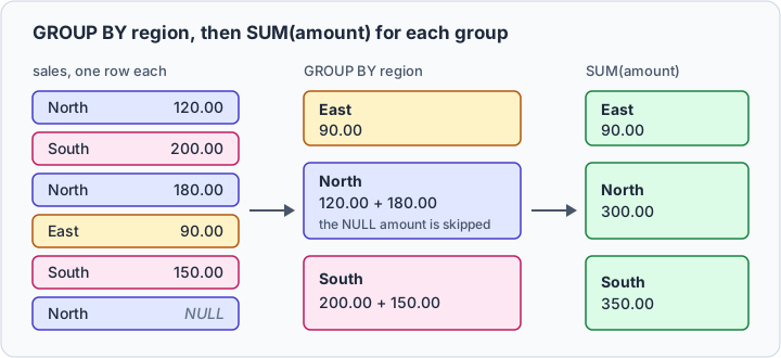
A SELECT list can hold every aggregate the report needs, and the database computes all of them over the same groups:
SELECT
    region,
    COUNT(*)              AS orders,
    MIN(amount)           AS min_sale,
    MAX(amount)           AS max_sale,
    SUM(amount)           AS total,
    ROUND(AVG(amount), 2) AS average
FROM sales
WHERE amount IS NOT NULL
GROUP BY region
ORDER BY total DESC;
| region | orders | min_sale | max_sale | total | average |
|---|---|---|---|---|---|
| South | 2 | 150.00 | 200.00 | 350.00 | 175.00 |
| North | 2 | 120.00 | 180.00 | 300.00 | 150.00 |
| East | 1 | 90.00 | 90.00 | 90.00 | 90.00 |
WHERE removed the row with no amount before the grouping, so COUNT(*) shows two orders for North rather than three.
WHERE cannot test an aggregate, because when it runs the groups do not exist yet. Write WHERE SUM(amount) > 100 and each engine refuses:
- PostgreSQL:
ERROR: aggregate functions are not allowed in WHERE - MySQL:
ERROR 1111 (HY000): Invalid use of group function - SQLite:
misuse of aggregate: SUM()
The clause for a condition on an aggregate is HAVING, which filters the groups after the aggregate has been computed:
SELECT region, SUM(amount) AS total
FROM sales
GROUP BY region
HAVING SUM(amount) > 100
ORDER BY total DESC;
| region | total |
|---|---|
| South | 350.00 |
| North | 300.00 |
East is gone: its whole group adds up to 90.00. Each clause has its own article, SQL GROUP BY Explained and SQL HAVING Clause.
A condition on one aggregate with FILTER or CASE
Sometimes only one aggregate should see a subset of the rows: the total of all sales and the total of North, side by side. WHERE cannot do it, because it applies to the whole query. The FILTER clause attaches a condition to one aggregate: only the rows for which the condition is true are fed to that function (PostgreSQL 17 documentation).
SELECT
    SUM(amount)                                 AS total_all,
    SUM(amount) FILTER (WHERE region = 'North') AS north_total,
    COUNT(*) FILTER (WHERE amount >= 150)       AS high_value_orders
FROM sales;
| total_all | north_total | high_value_orders |
|---|---|---|
| 740.00 | 300.00 | 3 |
PostgreSQL and SQLite run it. MySQL 9.1.0 stops with ERROR 1064 (42000), a syntax error at (WHERE region = 'North'). A CASE expression inside the aggregate does the same job on all three engines:
SELECT
    SUM(amount)                                     AS total_all,
    SUM(CASE WHEN region = 'North' THEN amount END) AS north_total,
    COUNT(CASE WHEN amount >= 150 THEN 1 END)       AS high_value_orders
FROM sales;
It returns the same row. A CASE with no ELSE gives NULL for the rows that do not match, and SUM and COUNT(column) skip NULL. FILTER reads more clearly, and CASE runs everywhere, so pick CASE when the query has to move between engines.
Subtotals with ROLLUP, CUBE and GROUPING SETS
GROUP BY region, product returns one row per pair that exists. A report usually wants the subtotal of each region and the grand total in the same result, and ROLLUP adds them: it groups by the list you give, then by each shorter prefix of it, down to no column at all (PostgreSQL 17 documentation).
SELECT region, product, SUM(amount) AS total
FROM sales
WHERE amount IS NOT NULL
GROUP BY ROLLUP(region, product)
ORDER BY region, product;
PostgreSQL returns:
| region | product | total |
|---|---|---|
| East | Widget | 90.00 |
| East | 90.00 | |
| North | Gadget | 180.00 |
| North | Widget | 120.00 |
| North | 300.00 | |
| South | Gadget | 200.00 |
| South | Widget | 150.00 |
| South | 350.00 | |
| 740.00 |
The rows with both columns filled are the plain GROUP BY region, product result. In the summary rows, the columns they do not group on hold NULL, which PostgreSQL sorts after every other value, so the grand total comes last. MySQL returns the same nine rows but sorts NULL first in ascending order (MySQL 8.4 manual), so its grand total is the first row. MySQL also accepts GROUP BY region, product WITH ROLLUP, which PostgreSQL rejects (MySQL 8.4 manual).
CUBE groups by every subset of the list instead of the prefixes, so GROUP BY CUBE(region, product) returns the nine rows above plus a total per product across all regions:
| region | product | total |
|---|---|---|
| Gadget | 380.00 | |
| Widget | 360.00 |
GROUPING SETS names the levels you want and nothing else. One total per region and one per product, with no pairs and no grand total:
SELECT region, product, SUM(amount) AS total
FROM sales
WHERE amount IS NOT NULL
GROUP BY GROUPING SETS ((region), (product))
ORDER BY region, product;
| region | product | total |
|---|---|---|
| East | 90.00 | |
| North | 300.00 | |
| South | 350.00 | |
| Gadget | 380.00 | |
| Widget | 360.00 |
The three engines support different parts of this, so check yours before you build a report on it:
| Clause | PostgreSQL 17.9 | MySQL 9.1.0 | SQLite 3.50.4 |
|---|---|---|---|
ROLLUP(...) | runs | runs | no such function: ROLLUP |
WITH ROLLUP | syntax error | runs | syntax error |
CUBE(...) | runs | ERROR 3889 | no such function: CUBE |
GROUPING SETS | runs | ERROR 1064 | syntax error |
What NULL does to each function
Every function except COUNT(*) skips a NULL rather than reading it as zero, as the table at the top shows. AVG is where that matters most, because the skipped row leaves the divisor as well as the total. COALESCE puts it back as a zero when zero is the right reading of a missing value:
SELECT
    ROUND(AVG(amount), 2)              AS avg_recorded,
    ROUND(AVG(COALESCE(amount, 0)), 2) AS avg_including_missing
FROM sales;
| avg_recorded | avg_including_missing |
|---|---|
| 148.00 | 123.33 |
The first is 740.00 divided by 5, the second the same 740.00 divided by 6. Both are correct, and they answer different questions, so label the column with the one your report asks. If nullable columns are new to you, see SQL NULL Values.
Aggregate functions vs window functions
A grouped aggregate replaces the rows it read with one row. A window function keeps every row and adds the summary next to it, which is what you need to show a sale and its region's total together:
SELECT sale_id, region, amount,
       SUM(amount) OVER (PARTITION BY region) AS region_total
FROM sales
WHERE amount IS NOT NULL
ORDER BY region, sale_id;
| sale_id | region | amount | region_total |
|---|---|---|---|
| 4 | East | 90.00 | 90.00 |
| 1 | North | 120.00 | 300.00 |
| 3 | North | 180.00 | 300.00 |
| 2 | South | 200.00 | 350.00 |
| 5 | South | 150.00 | 350.00 |
PARTITION BY region plays the part of GROUP BY, and five rows go in and five come out. Use the grouped form when one row per group is the answer, and the window form when each row has to stay. Window Functions in SQL covers the second in depth.
Mistakes that change the number you get
The first is a column in the SELECT list that is neither aggregated nor in GROUP BY. A group has no single value for it, and the engines disagree on what to do:
SELECT region, product, SUM(amount) AS total
FROM sales
GROUP BY region
ORDER BY region;
PostgreSQL refuses with column "sales.product" must appear in the GROUP BY clause or be used in an aggregate function. MySQL 9.1.0 refuses too, with ERROR 1055 (42000), because its default sql_mode includes ONLY_FULL_GROUP_BY (MySQL 8.4 manual). SQLite runs it and takes product from one row of each group (SQLite documentation):
| region | product | total |
|---|---|---|
| East | Widget | 90 |
| North | Widget | 300 |
| South | Gadget | 350 |
North's 300 includes a Gadget sale, yet the row says Widget. The fix is the same everywhere: add the column to GROUP BY for finer groups, or wrap it in an aggregate.
The second is a row-level condition, such as region = 'North', written into HAVING. Put it in WHERE, which runs before the grouping, so the database never builds the groups it would throw away. Only a condition on an aggregate has to stay in HAVING. For more examples of the counting functions, see SQL COUNT, AVG, and SUM Functions.
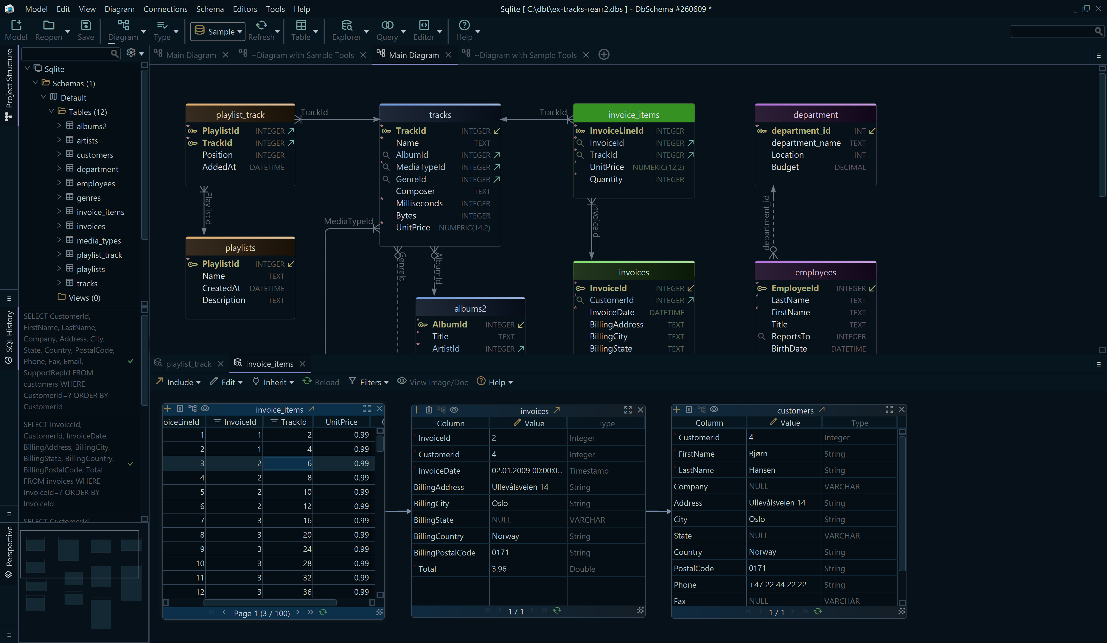
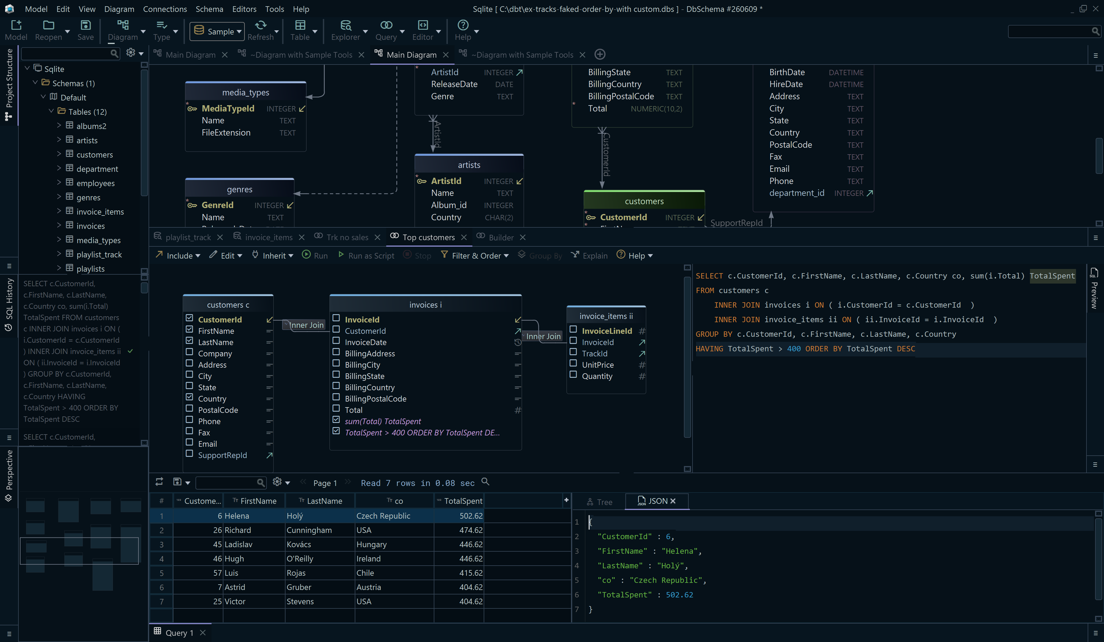

Build aggregate queries in DbSchema
The DbSchema Query Builder writes the aggregates and the GROUP BY list for you while you click. Right-click a table on the diagram and choose Query Editor, which is what the menus call the Query Builder. Tick the columns you want, then right-click a column and choose Aggregate → Sum(?), or Min(?), Max(?), Count(*), Count( distinct ?) or Avg(?). DbSchema adds a GROUP BY over the other ticked columns.
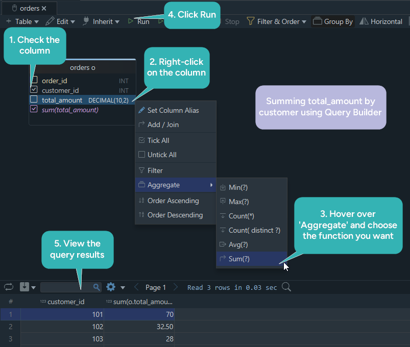
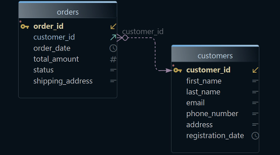
The SQL at the right changes with every click, and Run fills the result grid under the builder. Below, customers is joined to orders, with count(*) and a filter on status, and the generated query ends in a GROUP BY over the two name columns:
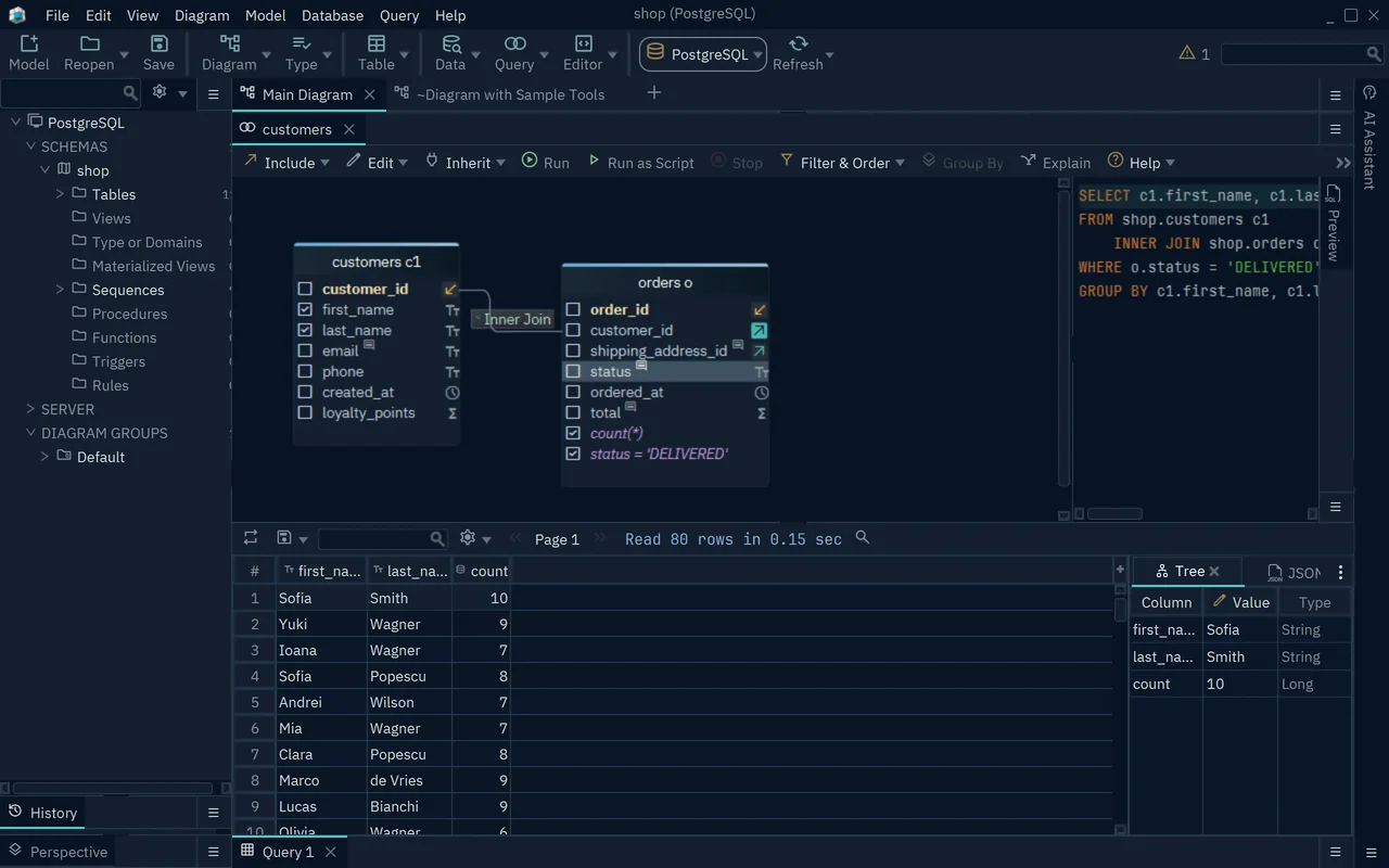
The builder only reads: a SELECT changes nothing in the database. When you close it, DbSchema asks whether to save the query to the project. Save and Close keeps it, and Query → Reopen opens it again.
Every query on this page runs as written in the DbSchema SQL Editor, which is in the free Community Edition: open it with Query → SQL Editor, paste a statement and press Run. The Query Builder, which writes the grouping list and the aggregates for you, needs DbSchema Pro. Download DbSchema from https://dbschema.com/download.html, connect to your database, and run the GROUP BY example against one of your own tables.
FAQ
Can SUM and AVG run on a text column?
PostgreSQL 17.9 rejects SUM(region) with function sum(character varying) does not exist, because no text type is among the inputs SUM and AVG accept (PostgreSQL 17 documentation). MySQL 9.1.0 returns 0 with warning 1292, Truncated incorrect DOUBLE value: 'North', and SQLite 3.50.4 returns 0.0. MIN and MAX read text on all three: MIN(region) is East and MAX(product) is Widget.
What does an aggregate function return when no rows match?
COUNT(*) and COUNT(column) return 0, while SUM, AVG, MIN and MAX return NULL on all three engines. Write COALESCE(SUM(amount), 0) when the report should show 0 (PostgreSQL 17 documentation).