Improve Performance with Range Partitioning in PostgreSQL
For a developer whose PostgreSQL table has grown large enough that a query about last month reads years of rows; every statement is shown with its result.
On this page
A table that has collected rows for years answers a question about last month by reading all of those years, unless something tells the planner where the rows for last month are. Range partitioning is one way to tell it: you split the table into child tables by the value of a column, PostgreSQL routes each new row into the child whose range covers it, and a query with a condition on that column reads only the children that can hold a match.
PostgreSQL 18 offers range, list and hash partitioning. The examples below use range, which is the one that fits a date.
What range partitioning does with the rows
Each partition covers an interval of the partitioning column, and the intervals may not overlap. The bounds are asymmetric, which is the detail that decides where a row on a boundary goes: the lower bound is inclusive and the upper bound is exclusive, so with one partition running from 1 to 10 and the next from 10 to 20, the value 10 belongs to the second.
Two things follow from the split. A query whose WHERE clause rules out a partition never reads that partition, which is what makes the table faster to query as it grows. And a year that is no longer needed is one table to detach and drop, rather than a DELETE of every row from that year followed by a VACUUM.
Both depend on picking the right column. It has to carry a value on every row at insert time, and it has to be the column your queries filter on, because a query that says nothing about it still reads every partition. A date column on a table that grows by date is the case where range partitioning pays, and it is the case shown here.
Create the parent table and its partitions
The parent declares the strategy and the column it partitions on:
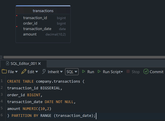
CREATE TABLE company.transactions (
  transaction_id BIGSERIAL,
  order_id BIGINT,
  transaction_date DATE NOT NULL,
  amount NUMERIC(10,2)
) PARTITION BY RANGE (transaction_date);
PARTITION BY RANGE (transaction_date) is the whole difference from an ordinary CREATE TABLE. From here the table accepts no rows at all until it has partitions to put them in. Each child names the parent and the range it takes:
CREATE TABLE company.transactions_before_2025
PARTITION OF company.transactions
FOR VALUES FROM (MINVALUE) TO ('2025-01-01');

CREATE TABLE company.transactions_2025
PARTITION OF company.transactions
FOR VALUES FROM ('2025-01-01') TO ('2026-01-01');
MINVALUE means there is no lower bound, so the first partition takes every date before 2025-01-01. The second takes 2025-01-01 itself and stops before 2026-01-01, by the inclusive-exclusive rule above. Nothing yet covers 2026, and a row from 2026 inserted now raises an error rather than landing somewhere arbitrary. If you would rather have a place for those rows than an error, add a partition declared DEFAULT, which collects every key value that fits no other partition.
The children are ordinary tables, and PostgreSQL links them to the parent through inheritance, so the catalog can list them:
SELECT c.relname AS partition_name
FROM pg_inherits i
JOIN pg_class c ON c.oid = i.inhrelid
WHERE i.inhparent = 'company.transactions'::regclass
ORDER BY 1;
| partition_name |
|---|
| transactions_2025 |
| transactions_before_2025 |
Insert rows and see where they land
Inserts go to the parent, exactly as they would to an unpartitioned table:
INSERT INTO company.transactions (order_id, transaction_date, amount) VALUES
(201, '2024-12-20', 450.00),
(202, '2025-01-15', 320.50),
(203, '2025-02-05', 125.00);
Nothing in the statement names a partition. PostgreSQL reads transaction_date on each row and puts the December 2024 row in transactions_before_2025 and the two 2025 rows in transactions_2025. Application code that was written before the table was partitioned keeps working unchanged.
The children can be queried directly, which is the quickest way to confirm the routing:
SELECT * FROM company.transactions_before_2025;
| transaction_id | order_id | transaction_date | amount |
|---|---|---|---|
| 1 | 201 | 2024-12-20 | 450.00 |
SELECT * FROM company.transactions_2025;
| transaction_id | order_id | transaction_date | amount |
|---|---|---|---|
| 2 | 202 | 2025-01-15 | 320.50 |
| 3 | 203 | 2025-02-05 | 125.00 |
The transaction_id values come from one sequence on the parent, so they run 1, 2, 3 across the partitions rather than starting again in each.
Query the partitioned table
Queries name the parent and read as they always did:
SELECT ROUND(SUM(amount), 2) AS total_amount
FROM company.transactions
WHERE transaction_date >= DATE '2025-01-01';
| total_amount |
|---|
| 445.50 |
The 450.00 from December is missing from the total because its partition was never read: the planner can see that transactions_before_2025 ends before 2025-01-01 and drops it from the plan. That behavior depends on enable_partition_pruning, which is on by default and is worth checking in postgresql.conf if a partitioned table is not getting faster.
Indexes follow the same pattern as the rows. Create one on the parent and PostgreSQL creates a matching index on every partition, including the partitions you add later, so each index covers one interval of dates instead of the whole history.
Pruning cuts both ways, though. A query that filters on order_id and says nothing about transaction_date gives the planner nothing to rule out, so it reads every partition and pays a little planning on top. Partitioning speeds up the queries that mention the partitioning column, and leaves the others where they were.
Add a partition for the next year
A range-partitioned table needs a new partition before the range it covers arrives:
CREATE TABLE company.transactions_2026
PARTITION OF company.transactions
FOR VALUES FROM ('2026-01-01') TO ('2027-01-01');
A table that already holds the right rows can join the parent instead of being created empty:
ALTER TABLE company.transactions
  ATTACH PARTITION company.transactions_2024
  FOR VALUES FROM ('2024-01-01') TO ('2025-01-01');
PostgreSQL scans that table before it accepts it, to check that every row in it belongs in the range you declared.
Old data leaves the same way it arrived:
ALTER TABLE company.transactions
  DETACH PARTITION company.transactions_before_2025;
The detached partition becomes a standalone table again, which you can dump, move to slower storage, or drop. This form takes an ACCESS EXCLUSIVE lock; adding CONCURRENTLY after DETACH PARTITION takes SHARE UPDATE EXCLUSIVE instead, so reads and writes carry on while it runs.
A partitioned table in DbSchema

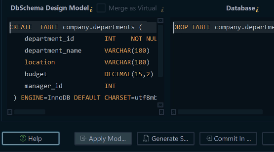
Every statement on this page runs in DbSchema's SQL Editor, the parent's CREATE TABLE included. Paste it in and click Execute Query, and the statement goes to the connected database. DbSchema then takes the new table into its own model and draws it on the diagram with its columns and types.
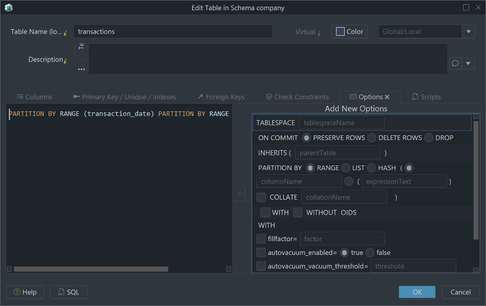
Once the table is drawn, double-click its header and DbSchema opens the Table Dialog on it. The Columns tab is the list of fields. The Options tab holds the database-specific table options, the ones DbSchema sets from the dialog instead of hand-written DDL. For company.transactions that tab carries the PARTITION BY RANGE (transaction_date) clause, as the screenshot below shows.
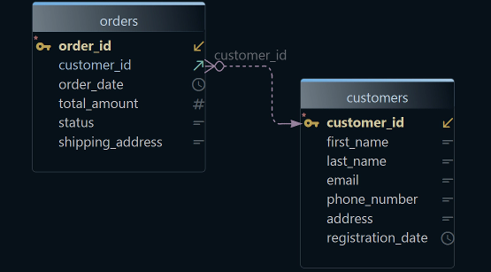
What the diagram shows is the parent. The children are not drawn beside it, and the way to see them is the pg_inherits query from earlier, run in the same DbSchema SQL Editor, where the result comes back as a grid. Between the two, the diagram tells you the table is partitioned and the query tells you what it is partitioned into.
Why the diagram still helps
A partitioned table is easy to misread from the SQL alone: a schema dump of a table partitioned by month shows a dozen tables with nearly the same name, and nothing in the list says that they are one table. In DbSchema the diagram shows the parent with its foreign keys, and the Options tab of its Table Dialog carries the partitioning clause, which is the part a reader of the schema actually needs.
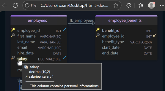
That answer also travels. Exporting HTML5 documentation from the diagram gives your team a page per table with the columns, the keys and the descriptions you wrote, so the partitioning is documented where everyone can read it rather than in the head of whoever set it up. When the design and the database drift apart, schema synchronization compares the two and generates the SQL for the differences, which you review before it runs.
The SQL Editor and the diagram are in the free DbSchema Community Edition, and the documentation export and schema synchronization are in Pro. Download it at https://dbschema.com/download.html, connect to the database that holds your largest table, and let DbSchema draw it on the diagram before you decide which column to partition it on.